This page is an add-on to the main page trilemmas. If the jargon below feels dense, learn the main principles first: the AI deploying trilemma (where the model lives), Blackwell is a family, model parallelism, long context is not free, knowledge engrams, cache offloading, prefill-decode disaggregation, MoE serving, and multi-token prediction.
They have different needs - this is real DC tokenomics with goodput.
Chat users send short prompts and judge you by one number: how fast the first token shows up. Agents fire long multi-turn workloads - huge contexts in, long generations out, many parallel calls at once. Each shape stresses the datacenter differently: chat is prefill-heavy bursts, agents hammer decode and the KV cache for minutes on end.
Raw tok/s is vanity; what a DC actually sells is goodput - tokens landing inside TTFT/TPOT SLOs per dollar of hardware. A GPU that is fast on paper but misses your latency targets produces zero goodput. That is why the config tables below differ per workload.
Today's MoEs are balanced - all experts are roughly the same size. Common misconception: a dedicated expert for coding and one for legal. Not true. To shard an LLM we want the opposite: the router picks many experts, nearly randomly, and the same set of experts can be loaded multiple times, so the load spreads across GPUs - hence the trend to more, smaller experts. More on this in the MoE sparsity section and the EP/MoE rows in the config maps below.
Draft a few tokens with a cheap model, verify them with the big one in a single pass - more tokens per second when drafts get accepted. It can be a built-in MTP head you just switch on, or an external drafter like EAGLE-3, DFlash 2 (parallel diffusion drafting), or DeepSeek's DSpark (dynamic scheduling adapts drafting to load). The message: different implementations have different perf and tradeoffs - extra memory for draft weights and cache, wasted compute on rejected drafts, and acceptance depends on the workload, so a wrong pick can be slower than no speculation at all.
SSM layers keep a compact fixed-size state instead of a growing KV cache, and a few attention layers stay in the mix for exact recall - smaller KV cache overall, smaller mem footprint. Qwen3.8-Flash-Next is exactly that: a GDN + QSA hybrid (3 of 4 layers Gated DeltaNet, the 4th Qwen Sparse Attention).
Main tricks: quantize, sparsify, page, offload, and sliding window + global dual attention - most layers only see a small recent window while a few global layers keep long-range recall, so the cache grows far slower than the context. The kicker: smaller cache = more things cached at once = more users and longer context on the same HBM. More volume with caching makes DC serving cheaper - that loop is DC tokenomics, the lever behind the big Dynamo-based configs in the InferenceX SemiAnalysis perf graphs.
Next stop - the InferenceX SemiAnalysis deep dive below: the perf-graph story (total tokens per $1 TCO vs P90 interactivity, every point has a story). The vLLM MiniMax-M3 recipe above documents the exact lane the graphs run. Configs first - graphs follow.
DC GPUs are in fact whole infra structure slices (simplified charging per slice used by NeoClouds). Rest of infra was at first not so important, but today it also serves KV cache, engram dictionary, agents, so looking deeper and understanding the whole infra is important.
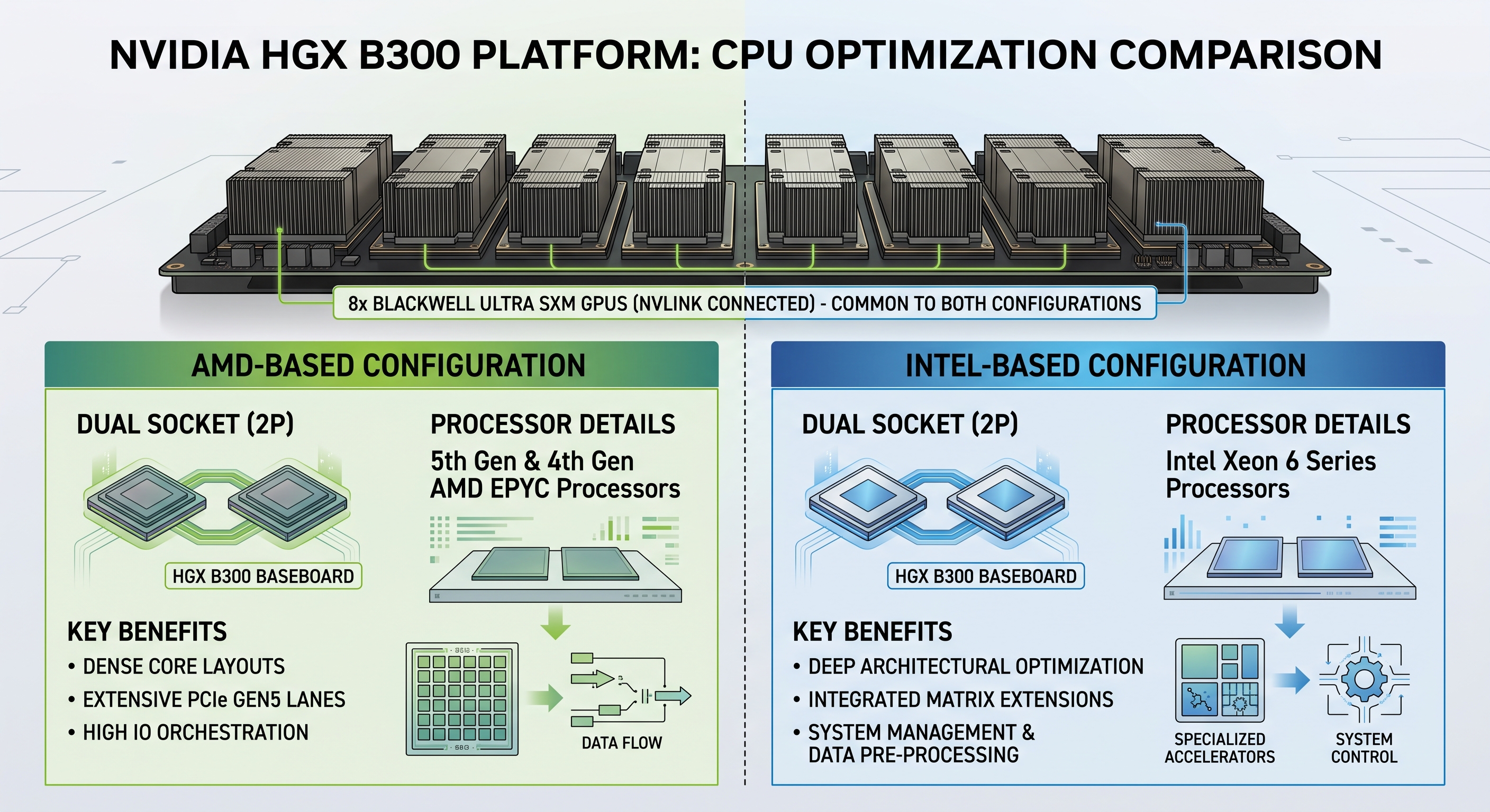
Coming in 8x GPU chassis (servers) with NVLink switch, small can be also 2x GPU NVLink bridge. The apples-vs-oranges part: DGX is the turnkey box you buy whole, HGX is the baseboard OEMs build their own servers on. The core is locked either way - 8x Blackwell, 1,440 GB (B200) / 2,300 GB (B300) HBM3e, 2x Xeon 8570, 14.4 TB/s NVLink. What you can configure around it: 2-4 TB RAM, ~30 TB NVMe cache, and ConnectX-7 or BlueField-3 NICs.
Can be custom configured for workload during production - not fully reproducible, but the plus is familiar x86 architecture - same CPUs (2x Xeon 8570) as the locked core above.
Not only GPU - a CPU (ARM) Grace with C2C NVLink, but many times in unified pods with nvidia networking, storage and so on - full nvidia recipe !!! 100% reproducibility. The NVL72 rack packs 36 Grace CPUs + 72 Blackwell GPUs into one 72-GPU NVLink domain with 130 TB/s NVLink bandwidth. GB300 Ultra goes further: 20 TB HBM3e, 1.5x FP4 and 2x attention throughput for reasoning workloads.
Unified and fully reproducible, but Grace CPU is ARM architecture - aarch64 only, so ops tooling and kernels must support it. The tradeoff mirrors the HGX side: reproducibility vs familiarity.
Notes:
See more in howto.hybridai.click - Automating HybridAI on NeoCloud with Agentic Infra approach
A model card is the official document the model authors ship with the model itself - usually as the Hugging Face repo page plus a linked technical report. It is the single source of truth for parameter counts (total vs active per token), context length, quantization and precision formats, hardware guidance and the license. Everything else is derived from it.
Why does it matter? Blog posts and vendor slides simplify. Engine teams (vLLM, SGLang) build their day-0 recipes straight from the model card and the linked technical report, so if a config works in a recipe, you can trace it back to card facts - not marketing.
Configs move fast, cards are the anchor. Before you reserve a GPU infra slice for any model below, recheck its card - numbers here were checked on 2026-09-01, but cards get updated as checkpoints and quantized variants ship.
Official model cards for all 6 models from the index list:
Model glance - 176B total parameters, ~6B active per token. The twist: 51B of the total is an N-gram embedding table that can live in host RAM and be prefetched asynchronously. Attention is a GDN + QSA hybrid (3 of 4 layers Gated DeltaNet, the 4th Qwen Sparse Attention). 262K native context, extensible to 1M with YaRN. Always reasons - thinking cannot be turned off.
| Engine | Hardware | Layout / precision | Validated on |
|---|---|---|---|
| vLLM | 2x GB300 (min) / 4x GB300 (full tray) | TP2 / TP4, FP8 | TP2 is the validated FP8 minimum; TP4 and TEP4 validated incl. MTP3 |
| vLLM | 8x H200 | TEP8, FP8 + Triton MoE | plain TP8 won't even load - incompatible with 128-wide FP8 quant blocks |
| vLLM | 4x MI355X | TP4, FP8 + AITER | ROCm path with VLLM_ROCM_USE_AITER=1 |
| vLLM | 1x B200/B300/GB300 (TP1) | TP1, NVFP4 | Blackwell-only quant; TP1 compile OOMs on GB300 - use TP2/TP4 |
| SGLang | 4x H200/B200/B300/GB300 | TP4, FP8; low-latency adds MTP (NEXTN) | high-throughput swaps in EP4, no spec decoding |
| SGLang | 8x MI350X/MI355X | TP8, FP8 + AITER | balanced strategy, page-size 32 |
--max-num-seqs 256 or the GDN recurrent-state cache errors at startup.Fireworks serves dedicated FP8 and NVFP4 deployments. Baseten - 404 at check time, recheck. Together - not yet, recheck.
Recipe sources - SGLang cookbook and vLLM recipe, plus NVIDIA GB300 NVL72 experiment blog.
Model glance - 428B total parameters, ~23B active per token (128 experts, 4 active per token). MiniMax Sparse Attention - a block-sparse "lightning indexer" that keeps long-context cost low (reported ~9x prefill / ~15x decode speedup over M2 at 1M context). 1M-token context. One quirk that shapes every config: --block-size 128 (SGLang: page-size 128) is mandatory on every platform - the MSA sparse/index cache must match.
| Engine | Hardware | Layout / precision | Validated on |
|---|---|---|---|
| vLLM | 8x H200 / H20 | TP8, BF16 | tight single-node BF16 fit; TP8+EP and DP8+EP variants too |
| vLLM | 8x B200 | TP8, NVFP4 | pair with EAGLE3 draft (MHA or GQA head, 3 spec tokens) |
| vLLM | MI300X/MI325X/MI355X | TP8, MXFP8/MXFP4 + AITER | MXFP8 runs from TP4 on gfx950; MI300X stacks accuracy-safe scheduling levers |
| SGLang | 8x H200 | TP8, BF16 | 1044 tok/s/GPU, GSM8K 97.0 |
| SGLang | 8x B200 | TP8, MXFP8 | 2385 tok/s/GPU, GSM8K 96.5 |
| SGLang | 4x B300 / GB300 | TP4, MXFP8 | 3285 tok/s/GPU on B300; 4323 tok/s/GPU on GB300 (8K-in/24-conc row) |
| SGLang | 8x MI3xx / MI355X | TP8, MXFP8 + AITER (TP4 on gfx950) | 420 tok/s/GPU on MI355X (1K-in/1K-out row) |
PD disaggregation - validated presets (the only model of the two with them)
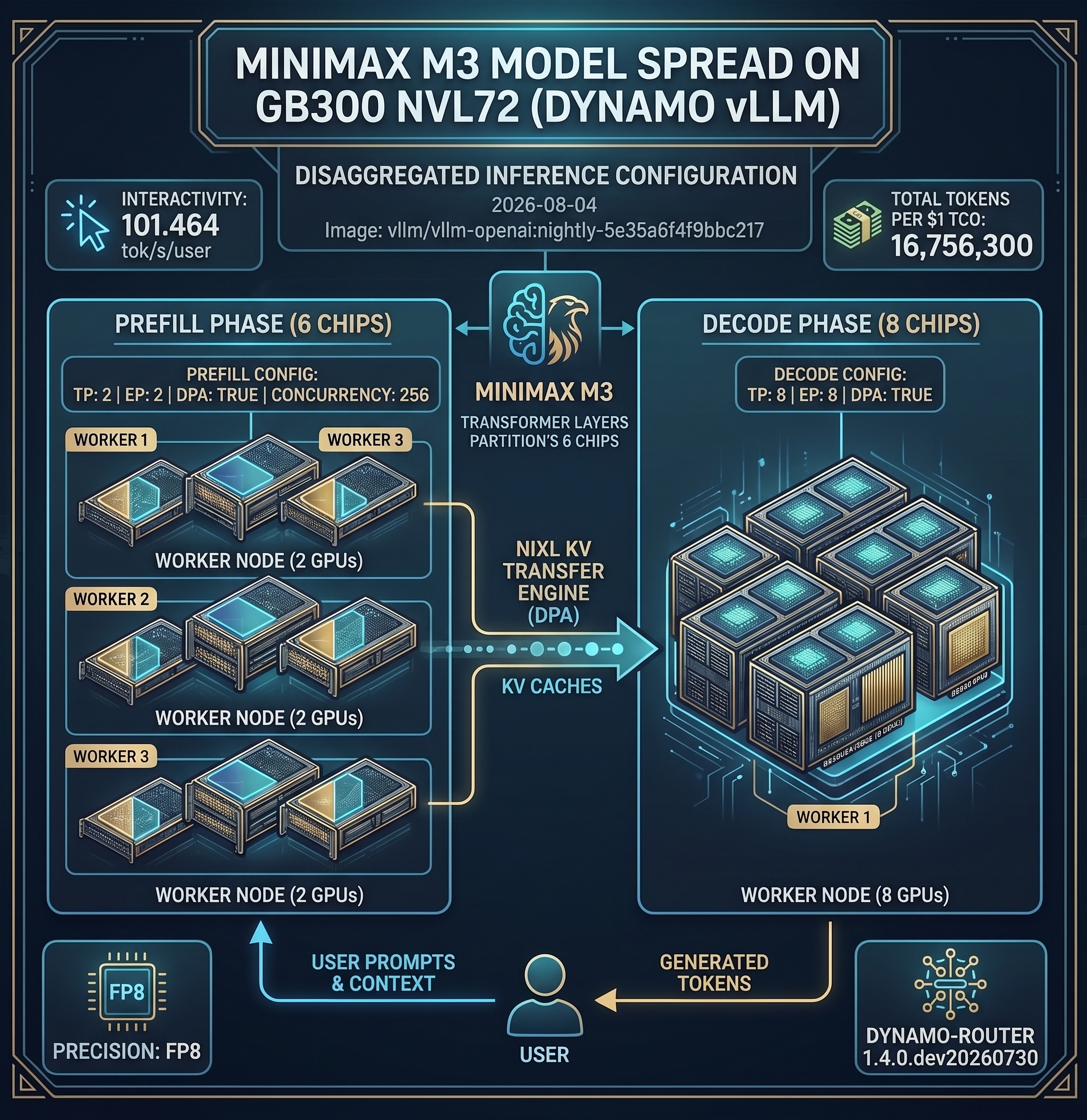
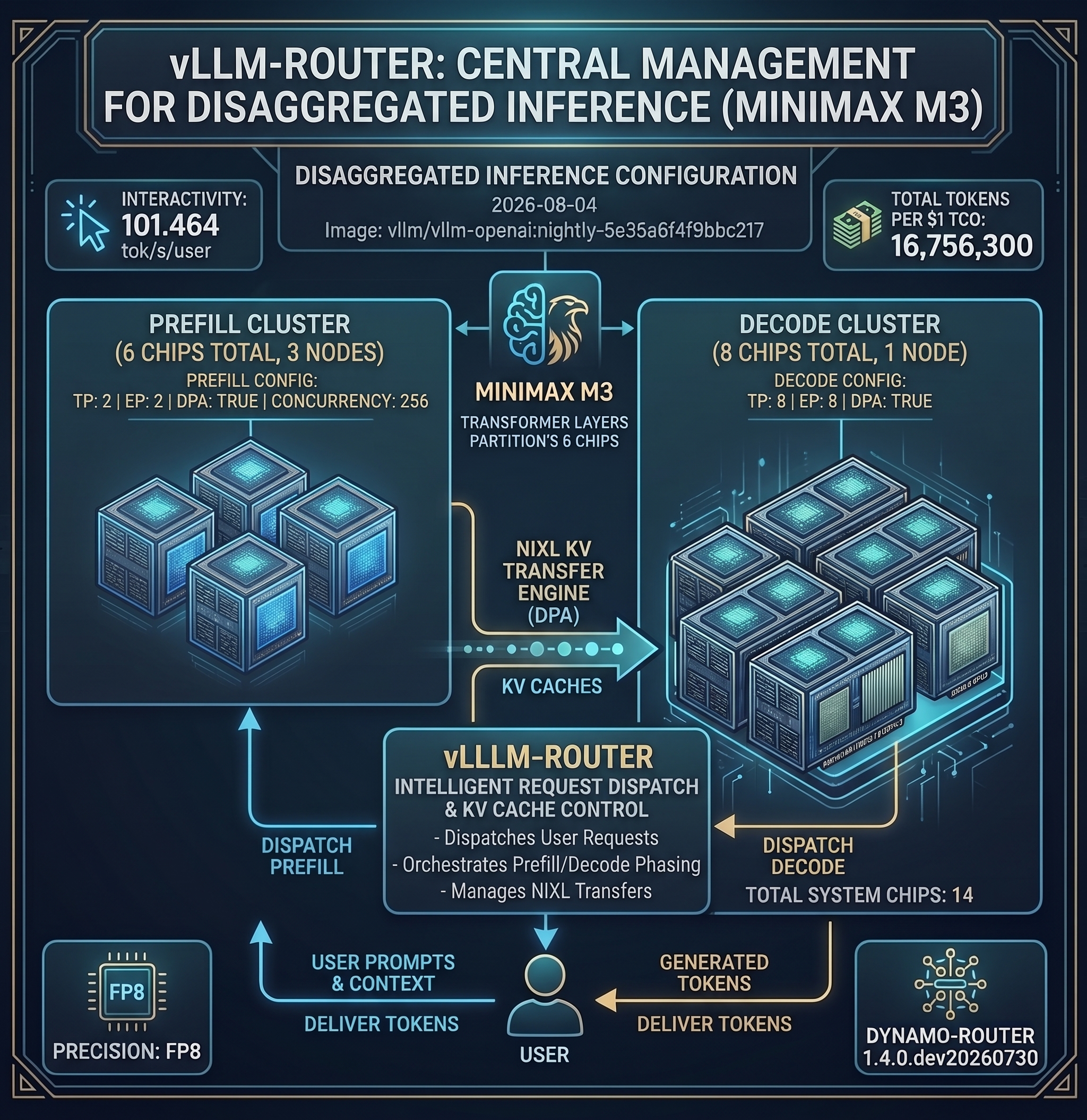
M3 runs prefill and decode on separate SGLang servers linked by an RDMA KV-transfer fabric (mooncake or NIXL), fronted by the PD router. The MSA-specific bit: every sparse lightning-indexer layer keeps a K-only index buffer that must reach the decode server too - SGLang transfers it alongside the main KV with no extra flags.
Fireworks serves serverless up to 512K context with public perf targets (TTFT P50 1 s / P90 6 s). Together serves 1M context serverless and dedicated. Baseten offers it in the Model API (no published configs).
Recipe sources - SGLang cookbook and vLLM recipe, plus Together AI serving blog.
InferenceX is SemiAnalysis's open-source agentic inference benchmark (inferencex.semianalysis.com, API at inferencex.semianalysis.com/api, code and recipes in github.com/SemiAnalysisAI/InferenceX). Why it is our golden etalon: every dashboard point comes from a public GitHub Actions run on real hardware, every config is a committed shell-script recipe in the repo, and the full benchmark database ships as weekly public snapshots - fully reproducible, auditable, open.
The same weights get served on everything from single 8x-GPU servers (H200, B200, B300) to whole-rack 72-GPU NVL72 pods from the full nvidia combos section - the apples-vs-oranges rule applies to benchmark charts too: compare graphs only per hardware slice. We focus on Nvidia; H200 and the Blackwell range - H100 and other platforms are niche in EU (Europe).
Tensor Parallel, Expert Parallel, Data Parallel (TP, EP, DP) - TP allows for maximize interactivity at small batch sizes, but it must carry out an all-reduce at every layer. EP shards experts, exploiting MoE sparsity, with the drawback being an all-to-all collective (which is more costly than simpler collectives like all-reduce) is carried out for MoE layers and can be imbalanced at small batches. DP replicates the entire model (or just parts of a model, like attention) on multiple groups of GPUs (ranks) and then load balances requests among ranks. It is the simplest to scale, but repeats weight loading which can be wasteful at scale.
Disaggregated Prefill - Disaggregated prefill (aka PD disaggregation or simply "disagg") is the practice of separating the prefill and decode phases across separate pools of GPUs or clusters. These separate prefill and decode pools can be tuned independently and scaled to match the needs of workloads.
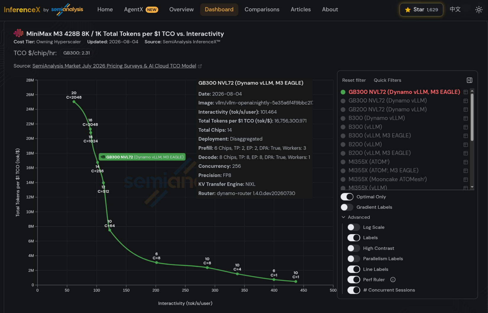
Past tests were synthetic perf loads (1k/1k and 8k/8k fixed shapes); now the dashboard runs AgentX scenarios - long-context, multi-turn agentic traces that hammer prefill, decode and the KV cache the way agents do (ties back to serving many users). The charts pit an SLO slider (tok/s per user) against cost per million total tokens - one axis per family: interactivity vs tokenomics. No price deep dive here, the shape of the tradeoff is the lesson.
The InferenceX dashboard is our main interest - lots of configs with git recipes, but without reasons for such large configs; we will address that specifically.
The fundamental tradeoff with LLM inference is throughput versus latency. Interactivity (tok/s/user) describes how fast each user of a system receives tokens - it is the inverse of time per output token (TPOT). Throughput (tok/s) describes how many total tokens a system can crank out across all users. One can achieve higher total throughput by batching requests, but each request will be allocated less FLOPs and thus complete slower. This is analogous to the choice of riding a metro bus vs a race car. The metro bus serves many riders, but also makes frequent stops, which takes time, but the cost of the metro bus can be amortized across many passengers. The race car can only carry one or two passengers, but it will make few if any additional stops meaning a faster travel time overall, but it is much more expensive to ride per passenger. The metro bus might make more sense for people heading to the park on a weekend, while the race car might be better for bringing a celebrity to their destination. There is no one-size-fits-all solution.
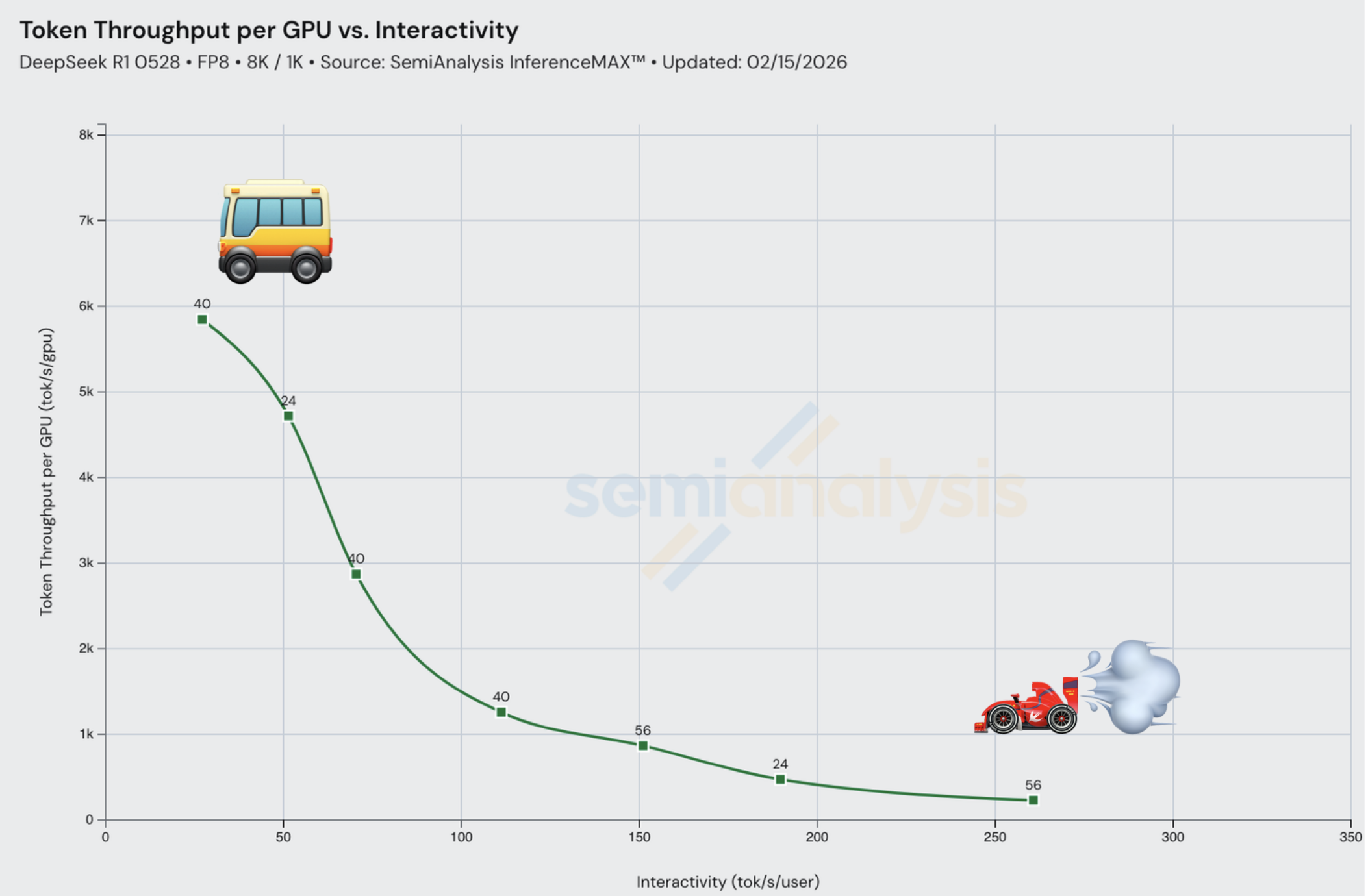
Image source: SemiAnalysis
Most benchmark results we will show in this article are an InferenceX curve. It is important to analyze throughput at various levels of interactivity/latency instead of just looking at maximum achieved throughput (which normally can only be achieved at a single low interactivity). With inference, there is no one-size-fits-all use case. The level of interactivity and throughput needed depends on the use case. For instance, real-time speech models require extremely low latency so that the end user can maintain a natural "conversation" with the LLM, whereas a basic QA chatbot may allow for higher latency. We leave it up to the reader to look at the curve and apply this principle to identify where their use case falls on the throughput-interactivity curve.
The Cost/Perf per TCO vs Interactivity/End-to-End Latency curve mostly follows the Throughput vs Interactivity/End-to-End Latency Curve: more tokens/hour leads to a lower cost per token as fixed $/hour costs are amortized over more tokens produced.
X-axis metric - Interactivity, end-to-end latency, or Time To First Token (TTFT) + agentic scenarios also offer E2E Normalized Interactivity.
Interactivity measures how quickly tokens stream after generation begins: approximately 1 / inter-token latency (ITL). E2E Normalized Interactivity measures the effective token rate over the whole request, including time to first token (TTFT): output tokens / end-to-end latency, or approximately 1 / (ITL + TTFT / output tokens). Both use tok/s/user. The normalized value penalizes slow TTFT, especially for short responses. Here, "normalized" means normalized by output length; it is not a 0–1 score or a comparison with another system.
Y-axis metrics - what the dashboard can plot:
| Group | Y-axis metric |
|---|---|
| Throughput | Token Throughput per Chip |
| Input Token Throughput per Chip | |
| Output Token Throughput per Chip | |
| Token Throughput per All in Utility MW | |
| Input Token Throughput per All in Utility MW | |
| Output Token Throughput per All in Utility MW | |
| Token Revenue per GPU Hour | Token Revenue per GPU Hour |
| Total Tokens per $1 TCO | Total Tokens per $1 TCO (Owning - Hyperscaler) |
| Total Tokens per $1 TCO (Owning - Neocloud Giant) | |
| Total Tokens per $1 TCO (3 Year Rental) | |
| Output Tokens per $1 TCO | Output Tokens per $1 TCO (Owning - Hyperscaler) |
| Output Tokens per $1 TCO (Owning - Neocloud Giant) | |
| Output Tokens per $1 TCO (3 Year Rental) | |
| Input Tokens per $1 TCO | Input Tokens per $1 TCO (Owning - Hyperscaler) |
| Input Tokens per $1 TCO (Owning - Neocloud Giant) | |
| Input Tokens per $1 TCO (3 Year Rental) | |
| Cost per Million Total Tokens | Cost per Million Total Tokens (Owning - Hyperscaler) |
| Cost per Million Total Tokens (Owning - Neocloud Giant) | |
| Cost per Million Total Tokens (3 Year Rental) | |
| Cost per Million Output Tokens | Cost per Million Output Tokens (Owning - Hyperscaler) |
| Cost per Million Output Tokens (Owning - Neocloud Giant) | |
| Cost per Million Output Tokens (3 Year Rental) | |
| Cost per Million Input Tokens | Cost per Million Input Tokens (Owning - Hyperscaler) |
| Cost per Million Input Tokens (Owning - Neocloud Giant) | |
| Cost per Million Input Tokens (3 Year Rental) | |
| All-in Provisioned Energy per Token | All-in Provisioned Joules per Total Token |
| All-in Provisioned Joules per Output Token | |
| All-in Provisioned Joules per Input Token | |
| Measured Energy | Measured Prefill Power per Chip |
| Measured Decode Power per Chip | |
| Measured Average Power per Chip | |
| Measured Joules per Input Token | |
| Measured Prefill Joules per Input Token | |
| Measured Joules per Output Token | |
| Measured Decode Joules per Output Token | |
| Measured Joules per Token (incl. prompt) | |
| Measured Joules per Successful Query | |
| Measured Watt-hours per Successful Query | |
| Measured Average Power as Percent of TDP | |
| Custom User Values | Total Tokens per $1 TCO (Custom User Values) |
| Cost per Million Total Tokens (Custom User Values) | |
| Token Throughput per All in Utility MW (Custom User Values) |
Chip config - is compound selector as: HW Platform + Engine + Cache + speculative encoding.
Scenarios - are mouse over on GRAPF (use advanced to enrich graph)
One word, two very different jobs. Mixing them up makes vendor slides and engine jargon unreadable. One buys you FLOPS, the other fights the memory bottleneck.
Sparse tensor formats (COO, HiCOO and friends) are data structures that let the hardware skip zero blocks entirely - you store and compute only the nonzero stuff. This is the trick behind NVIDIA sparse tensor cores and the big FLOPS-advantage multipliers vendors love to put on slides (10x-class numbers show up there - take them as marketing best-case, structured sparsity usually lands closer to 2x).
Intro to Sparse Tensors and Spatially Sparse Neural Networks (Chris Choy):
The MoE flavor of sparsity is about the bandwidth wall, not FLOPS. A huge total weight set sits in HBM, but per token only a few experts wake up - so you read and compute only a tiny slice of the weights instead of streaming all of them. Less weight traffic per token is how MoE fights the HBM bandwidth wall that caps decode speed (TPOT).
A Visual Guide to Mixture of Experts (MoE) in LLMs (Maarten Grootendorst):
The EP/MoE rows in the config maps are concept 2 - expert-parallel sharding works because only a few experts are active per token. The sparse attention indexers (Qwen QSA, the MiniMax-M3 lightning indexer) borrow concept 1's data-structure tricks to cut memory traffic on long context. Same word, different levers - now the jargon should read cleanly.
Qwen 3.8 Flash Next Tested: Is it Actually Fast?
MiniMax M3 explained in 8 min:
The Insane Infrastructure Design of DeepSeek V4:
Kimi K3 Architecture Explained - how the world's largest open-weight AI model works:
Modern Transformer Architecture Explained - But What Are Transformers?:
All configs above were checked on 2026-09-01. The recipes move fast (day-0 models, nightly images) - recheck before reserving hardware.